Carbon accounting underpins national carbon pricing and emissions trading schemes (ETS). However, without an international carbon pricing regime or carbon market, existing carbon accounting systems only reflect national accounting priorities and therefore vary in their approach to measuring emissions. Put simply, these systems aren’t designed to be comparable or even interoperable, rendering them ineffective for “apples to apples” comparisons of embodied greenhouse gas (GHG) emissions in goods that are traded across borders. As a result, and as countries start moving toward the adoption of carbon border adjustment mechanisms (CBAM) and eventually carbon clubs, the status quo patchwork of domestic schemes does not provide comparable measures of emissions content at the product level, a prerequisite for taxing goods at the border. A new carbon accounting paradigm that is specific to trade in goods must be created that resolves this disparity. Aligning carbon accounting with the Harmonized Tariff System (HTS), the international system of recognizing and classifying traded products for tariff collection, is therefore paramount to marrying trade and carbon accounting within this new paradigm.

In our last blog, we explored the differences in carbon accounting systems and how those systems lead to vastly different amounts of carbon emissions being attributed to the production of a single coffee cup. Here, we’re taking a deeper dive into the differences between the European Union (EU) ETS and the California ETS, because they are two functioning systems designed to be fit for trade purposes. However, even these schemes take such divergent approaches to measuring emissions that, all else being equal, the respective emissions calculations applied to annual raw steel production leads to substantially different results. In a world where the same steel product is traded across borders and divergent carbon measurements are used to calculate the border tax of steel, the value will be skewed—in both directions. Let us explain.

Comparing the European Union ETS & California ETS

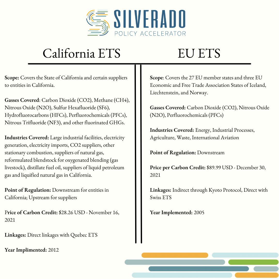
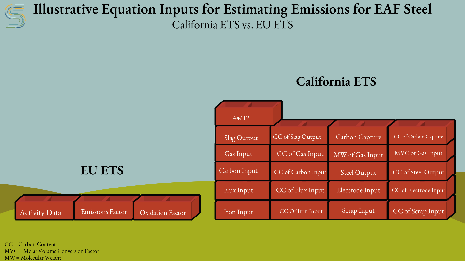
The EU ETS and California ETS both use a cap-and-trade system, and each use different forms of carbon accounting that companies employ on an annual basis to verify the amount of carbon credits they need to purchase to cover their emissions. The EU ETS calculates using basic emissions (i.e. GHG that is emitted during manufacturing, so call, ‘end-of-pipe’ emissions) and oxidation factors (i.e. the actual amount of fuel combusted during industrial processes). The California ETS uses a complex formula that multiplies inputs by their carbon content, including specifications for the molecular weight and volume of gas inputs. How an equation is structured is important–it’s like building a wall, where each brick adds to the stability of the overall structure - let’s look at how the California and EU systems compare. The EU’s simplified system of carbon accounting does not take into account as many factors as the California ETS, which, as one might expect, will lead to different results when each system is applied to the same product. See the below illustration showing the EAF steel equations used by the EU ETS compared to the California ETS, where one brick represents one variable within the equation.

To illustrate this point, we applied both the California ETS and EU-ETS to a scenario for annual raw steel production. Assuming that steel is produced either through an electric arc furnace (EAF) or a blast oxygen furnace (BOF) and that each production method accounts for 50% of an equal annual output of steel between the EU and California, the graphic below illustrates the outcomes for total emissions per one ton of raw steel between the two systems:

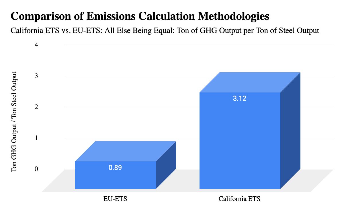
In theory, both the California ETS and EU ETS should yield similar results because they both represent 50% of total emissions under this scenario. Nonetheless, the EU’s share of emissions under its accounting scheme is roughly one-quarter of California’s under its accounting scheme. The EU ETS relies mostly on default emissions and oxidation factors and does not separate equations by technology type, leading to a large difference in outcomes between it and California for identical products under identical manufacturing conditions.

A Patchwork of National ETS and Carbon Pricing Systems Falls Short When it Comes to International Trade - A New Paradigm is Needed

Now, imagine these equations were the basis for determining a fair carbon border tariff for steel that is either imported into the US from the EU or vice versa. The use of this “apples-to-oranges” comparison in international trade would result in a mismatched system of border fees that would, in effect, form a border wall to imports under some systems while creating a border hedgerow in others for identical products. Such carbon tariff inversions would let carbon escape by failing to fully account for carbon outputs across jurisdictions and by creating an incentive to game those differences through trade transactions.

As the world starts to adopt cross-border climate measures, ETS systems are simply not fit for purpose when applied to international trade. The intent of an ETS was to create a market to reduce carbon emissions, not track and tax products as they move along a global supply chain. Indeed, the EU recognizes this as it has proposed a CBAM for purposes of traded goods rather than use its ETS system. However, the EU’s proposal still does not fundamentally address the issue of interoperability since it is not scaled to the HTS and does not provide a common measure on which to base border fees. Moving forward, a new trade paradigm is needed that aligns to the HTS and allows for “apples-to-apples” comparisons at the product level. Linking international trade and climate policy will be essential for any emissions reduction strategy and will be essential for comparing emissions globally.